Pendulum on a Cart — Part 1: Modeling

Introduction

The inverted pendulum on a cart is one of those problems that shows up in almost every control engineering course, and for good reason. At first glance it looks deceptively simple: a rod balanced upright on a moving platform. In practice it packs in everything that makes control interesting (nonlinearity, instability, coupled dynamics, and limited actuator authority) in a package small enough to fit on a desk.

This is the first post in a series documenting my own build. The goal is to balance a pendulum upright using a stepper-motor-driven cart, an encoder on the pivot, and an LQR controller running on an embedded system. In this post I work through the physics: where the equations of motion come from, what simplifications the hardware allows, and how to linearise around the unstable equilibrium to get a state-space model. Later posts will cover system identification (fitting the model to measured data) and control design.

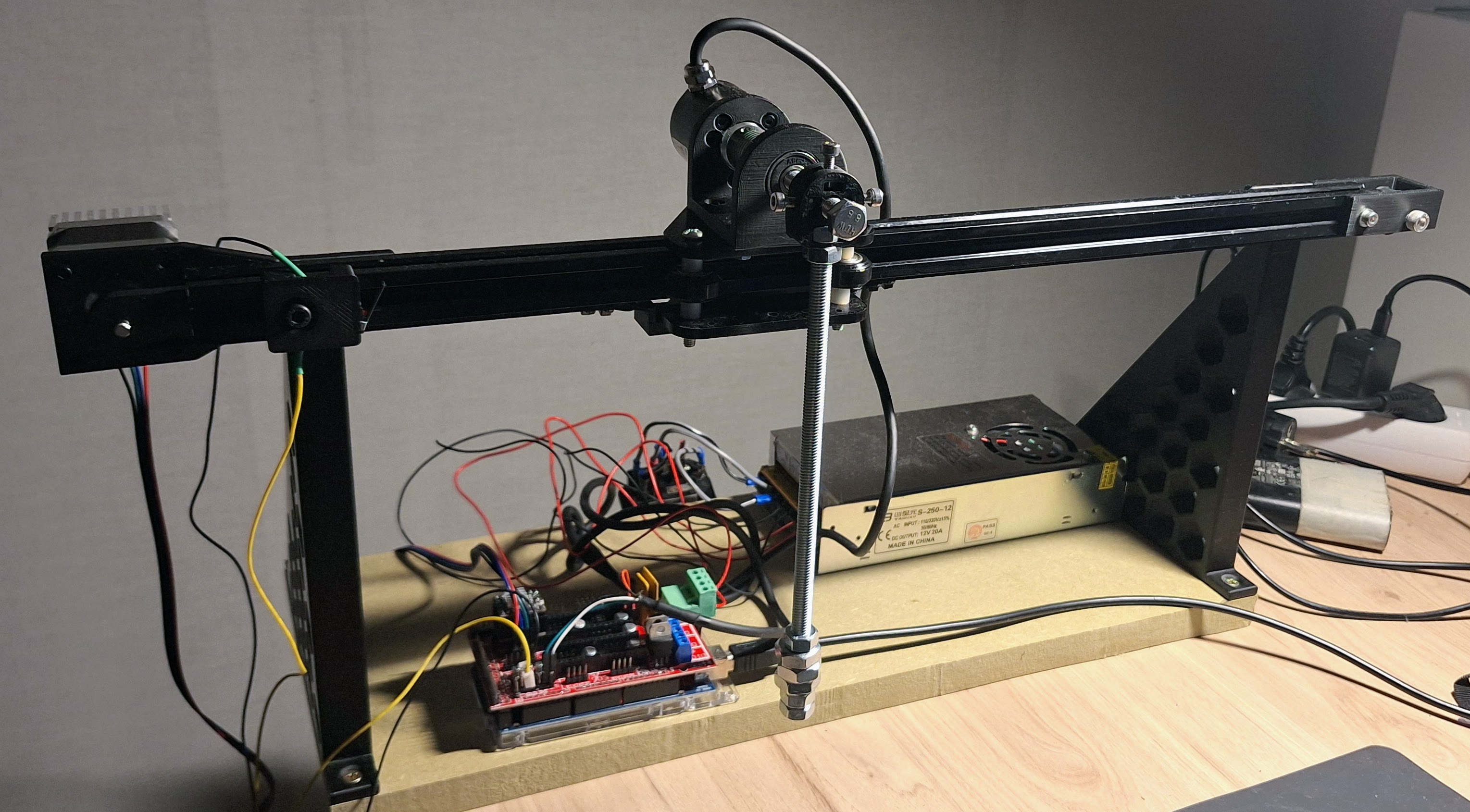The cart rides on a horizontal track driven by a stepper motor. An encoder at the pivot measures the pendulum angle.

System Description

The system has two degrees of freedom:

• \(x\) — horizontal position of the cart (positive to the right)
• \(\theta\) — angle of the pendulum measured from the downward vertical (so \(\theta = \pi\) is the upright position)

The cart has mass \(m_1\) and the pendulum is a uniform rod of mass \(m_2\) and length \(l\), pivoted at the top of the cart. An external horizontal force \(u\) acts on the cart.

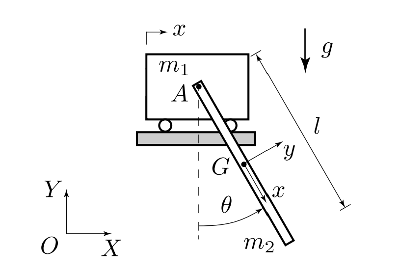System variables. The angle \(\theta\) is measured from the downward vertical, so the inverted equilibrium sits at \(\theta = \pi\).

For this derivation I assume no friction between the cart and the track, and no air resistance on the pendulum. Both of those get added back in later when we fit the model to data.

Lagrangian Mechanics — a quick primer

Newton’s laws are great when you can draw a clean free-body diagram. For a system like this (where the pendulum’s motion couples into the cart through the pivot) that gets messy fast. Lagrangian mechanics sidesteps the issue entirely by working with energies instead of forces.

The recipe is:

1. Write down the total kinetic energy \(T\) and potential energy \(V\) in terms of the generalised coordinates (here: \(x\) and \(\theta\)).
2. Form the Lagrangian \(\mathcal{L} = T - V\).
3. Apply the Euler-Lagrange equation for each coordinate \(q_i\):

\[\frac{d}{dt}\frac{\partial \mathcal{L}}{\partial \dot{q}_i} - \frac{\partial \mathcal{L}}{\partial q_i} = Q_i\]

where \(Q_i\) is the generalised force associated with coordinate \(q_i\). For \(q_1 = x\), the generalised force is the applied force \(u\). For \(q_2 = \theta\), there is no external torque, so \(Q_2 = 0\).

Deriving the Equations of Motion

Potential Energy

Only the pendulum contributes to the potential energy, since the cart moves horizontally and its height never changes. The centre of mass of the rod sits at \(l/2\) from the pivot. Its height above the pivot is \(\frac{l}{2}\cos\theta\), giving:

\[V = m_2 g \frac{l}{2} \cos\theta\]

Kinetic Energy

Cart. Pure translational motion:

\[T_\text{cart} = \frac{1}{2} m_1 \dot{x}^2\]

Pendulum. The kinetic energy of a rigid body is the sum of a translational part (motion of the centre of mass) and a rotational part (rotation about the centre of mass):

\[T_\text{pend} = \frac{1}{2} m_2 |\vec{v}_G|^2 + \frac{1}{2} J_G \dot{\theta}^2\]

where \(J_G = \frac{m_2 l^2}{12}\) is the moment of inertia of a uniform rod about its centre of mass.

Velocity of the centre of mass. This is the non-obvious part. The pivot point A moves with the cart at velocity \([\dot{x},\, 0]^T\) in the global frame. To find \(\vec{v}_G\) I work in the pendulum body frame, where the centre of mass is fixed at \(\vec{r}_{G/A} = [l/2,\, 0]^T\) (along the rod, away from the pivot).

The rotation matrix from the global frame to the pendulum frame (at \(\theta = 0\) the rod points straight down) is:

\[R_{bp} = \begin{bmatrix} \sin\theta & -\cos\theta \\ \cos\theta & \sin\theta \end{bmatrix}\]

The pivot velocity expressed in the pendulum frame:

\[\vec{v}_A^{(p)} = R_{bp} \begin{bmatrix} \dot{x} \\ 0 \end{bmatrix} = \begin{bmatrix} \dot{x}\sin\theta \\ \dot{x}\cos\theta \end{bmatrix}\]

Adding the contribution from the rod’s rotation (\(\dot{\theta}\,\hat{e}_z \times [l/2,\, 0]^T = [0,\, \dot{\theta}l/2]^T\)):

\[\vec{v}_G^{(p)} = \begin{bmatrix} \dot{x}\sin\theta \\ \dot{x}\cos\theta + \dot{\theta}\,l/2 \end{bmatrix}\]

Since the squared magnitude is frame-independent:

\[|\vec{v}_G|^2 = \dot{x}^2\sin^2\theta + \left(\dot{x}\cos\theta + \dot{\theta}\frac{l}{2}\right)^2 = \dot{x}^2 + l\,\dot{x}\dot{\theta}\cos\theta + \dot{\theta}^2\frac{l^2}{4}\]

Total kinetic energy. Substituting and collecting terms (and using \(\frac{l^2}{4} + \frac{l^2}{12} = \frac{l^2}{3}\) for a uniform rod):

\[T = \frac{1}{2}(m_1 + m_2)\dot{x}^2 + \frac{1}{2}m_2 l\,\dot{x}\dot{\theta}\cos\theta + \frac{1}{2}\frac{m_2 l^2}{3}\dot{\theta}^2\]

Lagrangian and Equations of Motion

\[\mathcal{L} = T - V = \frac{1}{2}(m_1+m_2)\dot{x}^2 + \frac{1}{2}m_2 l\,\dot{x}\dot{\theta}\cos\theta + \frac{1}{2}\frac{m_2 l^2}{3}\dot{\theta}^2 - m_2 g\frac{l}{2}\cos\theta\]

Applying the Euler-Lagrange equation for \(q_1 = x\):

\[\boxed{(m_1 + m_2)\ddot{x} + \frac{m_2 l}{2}\ddot{\theta}\cos\theta - \frac{m_2 l}{2}\dot{\theta}^2\sin\theta = u}\]

And for \(q_2 = \theta\):

\[\boxed{\frac{m_2 l^2}{3}\ddot{\theta} + \frac{m_2 l}{2}\ddot{x}\cos\theta + m_2 g\frac{l}{2}\sin\theta = 0}\]

These two coupled nonlinear ODEs fully describe the system dynamics.

Standard Manipulator Form

It is convenient to write the equations of motion in the compact matrix form used in robotics:

\[M(q)\ddot{q} + C(q,\dot{q})\dot{q} + G(q) + B\dot{q} = \tau\]

with \(q = [x,\, \theta]^T\) and \(\tau = [u,\, 0]^T\). The matrices are:

\[M(q) = \begin{bmatrix} m_1+m_2 & \frac{m_2 l}{2}\cos\theta \\ \frac{m_2 l}{2}\cos\theta & \frac{m_2 l^2}{3} \end{bmatrix}, \quad C(q,\dot{q}) = \begin{bmatrix} 0 & -\frac{m_2 l}{2}\dot{\theta}\sin\theta \\ 0 & 0 \end{bmatrix}\] \[G(q) = \begin{bmatrix} 0 \\ m_2 g\frac{l}{2}\sin\theta \end{bmatrix}, \quad B = \begin{bmatrix} b_1 & 0 \\ 0 & b_2 \end{bmatrix}\]

where \(b_1\) is the cart friction coefficient and \(b_2\) is the pivot friction coefficient. I set both to zero for the derivation above; they appear here because they will matter when fitting the model to real data.

From Full Model to Acceleration Input

Looking at the physical setup: the cart is driven by a stepper motor with enough torque that it can impose any commanded acceleration profile regardless of what the pendulum is doing. This changes things significantly.

In the full model, the first equation of motion (the cart equation) tells you how the force \(u\) is distributed between accelerating the cart and reacting to the pendulum’s push. With a stiff stepper, the motor internally generates whatever force is needed, so the cart acceleration \(\ddot{x}\) is no longer something to solve for: it is directly commanded. We relabel it as \(a\):

\[\ddot{x} = a\]

The first equation of motion becomes redundant and drops out. Only the pendulum equation survives:

\[\frac{m_2 l^2}{3}\ddot{\theta} + \frac{m_2 l}{2}\,a\cos\theta + m_2 g\frac{l}{2}\sin\theta = 0\]

Adding back the pivot friction \(b_2\dot{\theta}\) and rearranging for \(\ddot{\theta}\):

\[\ddot{\theta} = -\frac{3g}{2l}\sin\theta - \frac{b_2}{m_2 l^2/3}\dot{\theta} - \frac{3}{2l}\,a\cos\theta\]

Notice something: \(m_1\) and \(m_2\) have both disappeared. The pendulum dynamics depend only on the effective length \(l\), gravity \(g\), and the damping parameter. The cart mass is entirely absorbed into the stepper’s force budget. This is a direct consequence of having a stiff position-controlled actuator, and it is one of the reasons this hardware choice simplifies the control design so much.

Linearization Around the Inverted Equilibrium

The equation above is still nonlinear, so \(\sin\theta\) and \(\cos\theta\) prevent us from applying standard linear control tools directly. The trick is to linearise around the operating point we actually care about: the inverted equilibrium at \(\theta = \pi\), \(\dot{\theta} = 0\), \(a = 0\).

Define a small deviation from upright:

\[\varphi = \theta - \pi\]

For small \(\varphi\), the trigonometric functions simplify:

\[\sin\theta = \sin(\pi + \varphi) \approx -\varphi, \qquad \cos\theta = \cos(\pi + \varphi) \approx -1\]

Substituting into the pendulum equation:

\[\ddot{\varphi} = \frac{3g}{2l}\,\varphi - \frac{b_2}{m_2 l^2/3}\,\dot{\varphi} + \frac{3}{2l}\,a\]

To keep notation tidy, define:

\[L_\text{eff} = \frac{2l}{3}, \qquad b = \frac{b_2}{m_2 l^2/3}\]

Then:

\[\ddot{\varphi} = \frac{g}{L_\text{eff}}\,\varphi - b\,\dot{\varphi} + \frac{1}{L_\text{eff}}\,a\]

State-Space Model

With the state vector \(\mathbf{x}_s = [x,\; \dot{x},\; \varphi,\; \dot{\varphi}]^T\) and input \(a\), the linearised system is:

\[\dot{\mathbf{x}}_s = \underbrace{\begin{bmatrix} 0 & 1 & 0 & 0 \\ 0 & 0 & 0 & 0 \\ 0 & 0 & 0 & 1 \\ 0 & 0 & g/L_\text{eff} & -b \end{bmatrix}}_{A}\mathbf{x}_s + \underbrace{\begin{bmatrix} 0 \\ 1 \\ 0 \\ 1/L_\text{eff} \end{bmatrix}}_{B}a\]

The structure reveals something nice: the system splits cleanly into two blocks. Rows 1–2 describe the cart as a pure double integrator (\(\ddot{x} = a\)) with no pendulum coupling. Rows 3–4 describe the pendulum, with the cart acceleration \(a\) entering as a disturbance input. The only parameters that matter are \(L_\text{eff}\) (or equivalently \(l\)) and \(b\).

What’s Next

We have a linear state-space model, but it contains two unknown parameters: \(L_\text{eff}\) and \(b\). In Part 2 I’ll identify these from experimental data — first with a simple free-swing decay test, then with a more rigorous frequency sweep using the Best Linear Approximation framework.